The Discrete Time Convolution Calculator is a tool used to compute the convolution of two discrete-time signals. Convolution is a fundamental operation in signal processing, systems analysis, and control theory. It is used to determine the output of a system when given an input signal and the system's impulse response.
In discrete-time systems, the convolution operation helps to understand how an input sequence is transformed by the system's response. This is especially important in fields like digital signal processing, communications, and audio processing, where signals are manipulated to achieve desired effects or to filter out unwanted noise. The Discrete Time Convolution Calculator allows for quick and easy computation of the convolution, which is a core operation in many technical applications.
Formula of Discrete Time Convolution Calculator
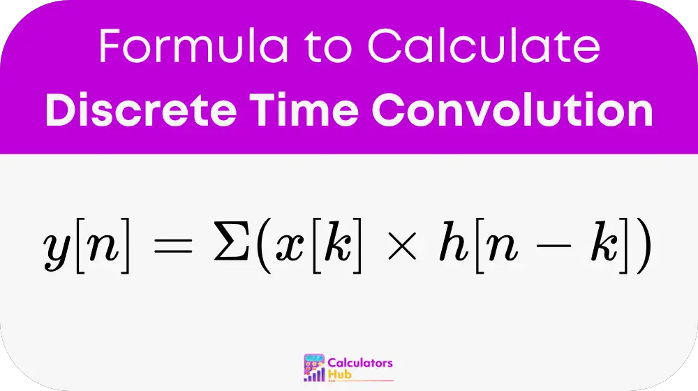
The general formula for Discrete Time Convolution is given by:
Where:
- y[n] = output sequence at time index n
- x[k] = input sequence at time index k
- h[n - k] = system's impulse response, shifted by n - k
- Σ = summation symbol, indicating that the sum is taken over all possible values of k where both sequences x[k] and h[n - k] are defined
Explanation of Terms:
- x[k] is the input signal or sequence that is being passed through the system.
- h[n - k] is the system's impulse response, which describes how the system reacts to an impulse at any point in time.
- The convolution process essentially "slides" the impulse response h[n - k] across the input sequence x[k], calculating the weighted sum of the products of overlapping values.
The convolution sum represents how the input signal x[k] is transformed by the system's impulse response h[n - k] over time.
General Terms for Discrete Time Convolution Calculation
The following table provides general terms and concepts that are essential for understanding the Discrete Time Convolution Calculator. These terms will help users who are new to convolution or signal processing:
| Term | Description |
|---|---|
| Discrete Time | A sequence of values indexed by discrete time intervals (e.g., n = 0, 1, 2, ...). |
| Convolution | A mathematical operation that combines two sequences to produce a third. |
| Impulse Response | The output of a system when the input is an impulse function (a single unit at time n=0). |
| Input Sequence (x[k]) | The sequence of values representing the input signal to the system. |
| Output Sequence (y[n]) | The resulting sequence after applying the convolution operation to the input and impulse response. |
| Summation (Σ) | The summing of the products of the input and impulse response over time indices. |
This table serves as a quick reference to the key concepts and components involved in discrete time convolution, making it easier to understand how the calculation is performed.
Example of Discrete Time Convolution Calculator
Let’s go through an example to demonstrate how the Discrete Time Convolution Calculator works.
Example 1: Convolution of Two Simple Sequences
Suppose we have the following input and impulse response sequences:
- Input sequence (x[k]): [1, 2, 3]
- Impulse response (h[k]): [0.5, 1]
We want to calculate the output sequence y[n] using the convolution formula.
Step 1: Write the Convolution Formula
Using the formula y[n] = Σ (x[k] * h[n - k]), we will calculate the convolution for each value of n.
Step 2: Calculate y[0]
For n = 0:
- y[0] = (x[0] * h[0 - 0]) + (x[1] * h[0 - 1])
- y[0] = (1 * 0.5) + (2 * 0) = 0.5
So, y[0] = 0.5.
Step 3: Calculate y[1]
For n = 1:
- y[1] = (x[0] * h[1 - 0]) + (x[1] * h[1 - 1]) + (x[2] * h[1 - 2])
- y[1] = (1 * 1) + (2 * 0.5) + (3 * 0) = 1 + 1 = 2
So, y[1] = 2.
Step 4: Calculate y[2]
For n = 2:
- y[2] = (x[0] * h[2 - 0]) + (x[1] * h[2 - 1]) + (x[2] * h[2 - 2])
- y[2] = (1 * 1) + (2 * 1) + (3 * 0.5) = 1 + 2 + 1.5 = 4.5
So, y[2] = 4.5.
Step 5: Final Output Sequence
The output sequence y[n] is [0.5, 2, 4.5]. This means that after passing the input sequence through the system characterized by the impulse response, the resulting output sequence is [0.5, 2, 4.5].
Most Common FAQs
Convolution plays a crucial role in signal processing, as it helps analyze how an input signal is modifie by a system's response. It is use in applications such as filtering, system analysis, and image processing. Convolution allows engineers and scientists to predict the behavior of systems when subjected to various signals.
The impulse response of a system depends on the nature of the system being analyzed. It can be determine experimentally or derived based on the system's characteristics. In practical applications, the impulse response could represent anything from an electronic filter to the characteristics of a physical system like a mechanical or acoustic device.
No, the Discrete Time Convolution Calculator is specifically design for discrete-time signals, where both the input and output sequences are represent by discrete time intervals. For continuous-time signals, you would need to use continuous-time convolution, which involves integrals instead of summations.